Asterisk - The Open Source VoIP PBX - Section 7.2. Digital Telephony

7.2. Digital Telephony

Analog telephony is almost dead.

In the PSTN, the famous Last Mile is the final remaining piece of the telephone network still using technology pioneered well over a hundred years ago.^[]

^[] "The Last Mile" is a term that was originally used to describe the only portion of the PSTN that had not been converted to fiber optics: the connection between the central office and the customer. The Last Mile is more than that, however, as it also has significance as a valuable asset of the traditional phone companiesthey own a connection into your home. The Last Mile is becoming more and more difficult to describe in technical terms, as there are now so many ways to connect the network to the customer. As a thing of strategic value to telecom, cable, and other utilities, its importance is obvious.

One of the primary challenges when transmitting analog signals is that all sorts of things can interfere with those signals, causing low volume, static, and all manner of other undesired effects. Instead of trying to preserve an analog waveform over distances that may span thousands of miles, why not simply measure the characteristics of the original sound and send that information to the far end? The original waveform wouldn't get there, but all the information needed to reconstruct it would.

This is the principle of all digital audio (including telephony): sample the characteristics of the source waveform, store the measured information, and send that data to the far end. Then, at the far end, use the transmitted information to generate a completely new audio signal that has the same characteristics as the original. The reproduction is so good that the human ear can't tell the difference.

The principle advantage of digital audio is that the sampled data can be mathematically checked for errors all along the route to its destination, ensuring that a perfect duplicate of the original arrives at the far end. Distance no longer affects quality, and interference can be detected and eliminated.

7.2.1. Pulse-Code Modulation

There are several ways to digitally encode audio, but the most common method (and the one used in telephony systems) is known as Pulse-Code Modulation (PCM). To illustrate how this works, let's go through a few examples.

7.2.1.1. Digitally encoding an analog waveform

The principle of PCM is that the amplitude of the analog waveform is sampled at specific intervals so that it can later be recreated. The amount of detail that is captured is dependent both on the bit-resolution of each sample and on how frequently the samples are taken. A higher bit-resolution and a higher sampling rate will provide greater accuracy, but more bandwidth will be required to transmit this more detailed information.

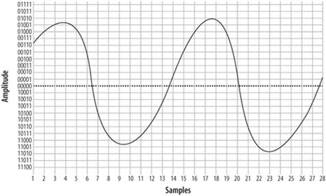
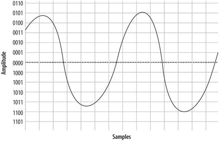
To get a better idea of how PCM works, consider the waveform displayed in Figure 7-2.

To digitally encode the wave, it must be sampled on a regular basis, and the amplitude of the wave at each moment in time must be measured. The process of slicing up a waveform into moments in time and measuring the energy at each moment is called quantization , or sampling.

The samples will need to be taken frequently enough and will need to capture enough information to ensure that the far end can recreate a sufficiently similar waveform. To achieve a more accurate sample, more bits will be required. To explain this concept, we will start with a very low resolution, using four bits to represent our amplitude. This will make it easier to visualize both the quantization process itself and the effect that resolution has on quality.

Figure 7-3 shows the information that will be captured when we sample our sine wave at four-bit resolution.

Figure 7-2. A simple sinusoidal (sine) wave

Figure 7-3. Sampling our sine wave using four bits

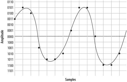
At each time interval, we measure the amplitude of the wave and record the corresponding intensityin other words, we sample it. You will notice that the four-bit resolution limits our accuracy. The first sample has to be rounded to 0011, and the next quantization yields a sample of 0101. Then comes 0100, followed by 1001, 1011, and so forth. In total, we have 14 samples (in reality, several thousand samples must be taken per second). If we string together all the values, we can send them to the other side as:

    0011 0101 0100 1001 1011 1011 1010 0001 0101 0101 0000 1100 1100 1010

On the wire, this code might look something like Figure 7-4.

Figure 7-4. PCM encoded waveform

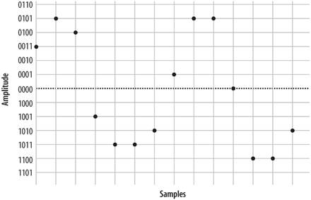
When the far end's digital-to-analog (D/A) converter receives this signal, it can use the information to plot the samples, as shown in Figure 7-5.

Figure 7-5. Plotted PCM signal

From this information, the waveform can be reconstructed (see Figure 7-6).

Figure 7-6. Delineated signal

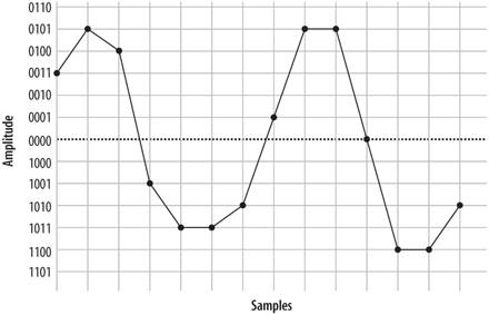
As you can see if you compare Figure 7-7 with Figure 7-8, this reconstruction of the waveform is not very accurate. This was done intentionally, to demonstrate an important point: the quality of the digitally encoded waveform is affected by the resolution and rate at which it is sampled. At too low a sampling rate, and with too low a sample resolution, the audio quality will not be acceptable.

7.2.1.2. Increasing the sampling resolution and rate

Let's take another look at our original waveform, this time using five bits to define our quantization intervals (Figure 7-7).

Figure 7-7. The same waveform, on a higher-resolution overlay

In reality, there is no such thing as five-bit PCM. In the telephone network, PCM samples are encoded using eight bits.^[*]

^[*] Other digital audio methods may employ 16 bits or more.

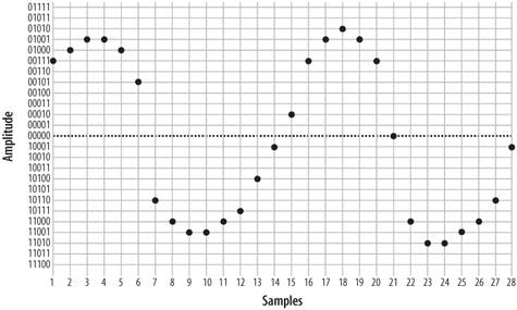
We'll also double our sampling frequency. The points plotted this time are shown in Figure 7-8.

We now have twice the number of samples, at twice the resolution. Here they are:

    00111 01000 01001 01001 01000 00101 10110 11000 11001 11001 11000 10111 
    10100 10001 00010 00111 01001 01010 01001 00111 00000 11000 11010 11010 
    11001 11000 10110 10001

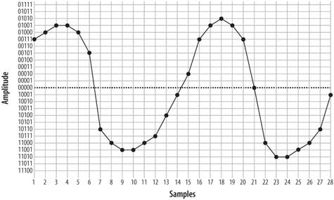
When received at the other end, that information can now be plotted as shown in Figure 7-9.

Figure 7-8. The same waveform at double the resolution

Figure 7-9. Five-bit plotted PCM signal

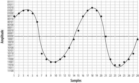
From this information, the waveform shown in Figure 7-10 can then be generated.

As you can see, the resultant waveform is a far more accurate representation of the original. However, you can also see that there is still room for improvement.

Note that 40 bits were required to encode the waveform at 4-bit resolution, while 156 bits were needed to send the same waveform using 5-bit resolution (and also doubling the sampling rate). The point is, there is a tradeoff: the higher the quality of audio you wish to encode, the more bits will be required to do it, and the more bits you wish to send (in real time, naturally), the more bandwidth you will need to consume.

Figure 7-10. Waveform delineated from five-bit PCM

7.2.1.3. Nyquist's Theorem

So how much sampling is enough? That very same question was considered in the 1920s by an electrical engineer (and AT&T/Bell employee) named Harry Nyquist. Nyquist's Theorem^[*] states: "When sampling a signal, the sampling frequency must be greater than twice the bandwidth of the input signal in order to be able to reconstruct the original perfectly from the sampled version."

^[*] Nyquist published two papers, "Certain Factors Affecting Telegraph Speed" (1924) and "Certain Topics in Telegraph Transmission Theory" (1928), in which he postulated what became known as Nyquist's Theorem. Proven in 1949 by Claude Shannon ("Communication in the Presence of Noise"), it is also referred to as the Nyquist-Shannon sampling theorem.

In essence, what this means is that to accurately encode an analog signal you have to sample it twice as often as the total bandwidth you wish to reproduce. Since the telephone network will not carry frequencies below 300 Hz and above 4,000 Hz, a sampling frequency of 8,000 samples per second will be sufficient to reproduce any frequency within the bandwidth of an analog telephone. Keep that 8,000 samples per second in mind; we're going to talk about it more later.

7.2.1.4. Logarithmic companding

So, we've gone over the basics of quantization, and we've discussed the fact that more quantization intervals (i.e., a higher sampling rate) give better quality but also require more bandwidth. Lastly, we've discussed the minimum sample rate needed to accurately measure the range of frequencies we wish to be able to transmit (in the case of the telephone, it's 8,000 Hz). This is all starting to add up to a fair bit of data being sent on the wire, so we're going to want to talk about companding.

Companding is a method of improving the dynamic range of a sampling method without losing important accuracy. It works by quantizing higher amplitudes in a much coarser fashion than lower amplitudes. In other words, if you yell into your phone, you will not be sampled as cleanly as you will be when speaking normally. Yelling is also not good for your blood pressure, so it's best to avoid it.

Two companding methods are commonly employed: m-law^[*] in North America, and A-law in the rest of the world. They operate on the same principles but are otherwise not compatible with each other.

^[*] m-law is often referred to as "u-law" because, let's face it, how many of us have m keys on our keyboards? m is in fact the Greek letter Mu; thus, you will also see m-law written (more correctly) as "Mu-law." When spoken, it is correct to confidently say "Mew-law," but if folks look at you strange, and you're feeling generous, you can help them out and tell them it's "u-law." Many people just don't appreciate trivia.

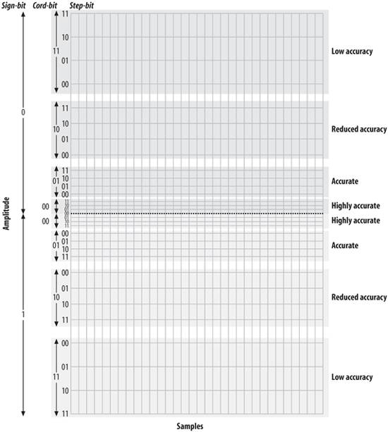
Companding divides the waveform into cords , each of which has several steps . Quantization involves matching the measured amplitude to an appropriate step within a cord. The value of the band and cord numbers (as well as the signpositive or negative) becomes the signal. The following diagrams will give you a visual idea of what companding does. They are not based on any standard, but rather were made up for the purpose of illustration (again, in the telephone network companding will be done at an eight-bit, not five-bit, resolution).

Figure 7-11 illustrates five-bit companding. As you can see, amplitudes near the zero-crossing point will be sampled far more accurately than higher amplitudes (either positive or negative). However, since the human ear, the transmitter, and the receiver will also tend to distort loud signals, this isn't really a problem.

A quantized sample might look like Figure 7-12. It yields the following bit stream:

    00000 10011 10100 10101 01101 00001 00011 11010 00010 00001 01000 10011 
    10100 10100 00101 00100 00101 10101 10011 10001 00011 00001 00000 10100 
    10010 10101 01101 10100 00101 11010 00100 00000 01000

7.2.1.5. Aliasing

If you've ever watched the wheels on a wagon turn backward in an old Western movie, you've seen the effects of aliasing . The frame rate of the movie cannot keep up with the rotational frequency of the spokes, and a false rotation is perceived.

In a digital audio system (which the modern PSTN arguably is), aliasing always occurs if frequencies that are greater than one-half the sampling rate are presented to the analog-to-digital (A/D) converter . In PSTN, that is any audio frequencies above 4,000 Hz (half the sampling rate of 8,000 Hz). This problem is easily corrected by passing the audio through a low-pass filter ^[] before presenting it to the A/D converter.

^[] A low-pass filter, as its name implies, allows through only frequencies that are lower than its cut-off frequency. Other types of filters are high-pass filters (which remove low frequencies) and band-pass filters (which filter out both high and low frequencies).